Introduction to Autoregressive (AR) Processes

Autoregressive (AR) processes are a class of time series models used to describe a variable that is correlated with its past values. AR models are widely applied in various fields such as economics, engineering, finance, and traffic modeling, among others. In this post, we will introduce the concept of AR processes, their mathematical formulation, and the different types of AR models used in time series forecasting.

What is an Autoregressive Process?

An Autoregressive (AR) process is a time series model where the current value of a variable is expressed as a linear function of its previous values plus a noise term (also known as error or residual). The AR model assumes that past values have a direct influence on the current value.

Key Characteristics of AR Processes:

1. Dependence on Past Values:
   • The primary idea behind AR processes is that the current value of a time series is influenced by its ** previous values**. This dependence can be seen as the “memory” of the system, which is useful for forecasting.
2. Linear Relationship:
   • The relationship between current and past values is assumed to be linear, which simplifies both modeling and computation.
3. Stationarity:
   • For an AR process to be valid, the time series must be stationary—i.e., its statistical properties, such as mean and variance, should remain constant over time. If the data is not stationary, it must be transformed (e.g., differencing) before applying AR models.

Mathematical Formulation of AR Processes

The simplest form of an AR model is the AR(1) process, which describes the current value of a time series as a function of the immediately preceding value.

AR(1) Process

An AR(1) process can be represented mathematically as:

Where:

• \(x_t\) is the current value at time \(t\),
• \(\phi_1\) is the autoregressive coefficient (the strength of dependence on the previous value),
• \(x_{t-1}\) is the previous value at time \(t-1\),
• \(\epsilon_t\) is the error term (also called white noise), which is assumed to be normally distributed with zero mean and constant variance: \(\epsilon_t \sim \mathcal{N}(0, \sigma^2)\).

Interpretation of Parameters:

• \(\phi_1\): This coefficient controls how much influence the previous value has on the current value. If \( |\phi_1| < 1\), the process is stable and will not diverge over time.
• \(\epsilon_t\): The error term represents random noise that is independent across time periods.

AR(p) Process

The general form of an AR(p) process, where \(p\) is the number of lags (past values) included, is:

where \(\phi_1, \phi_2, \dots, \phi_p\) are the autoregressive coefficients for the corresponding lags, \(p\) is the order of the process (i.e., how many previous time steps are included in the model).

import numpy as np
import matplotlib.pyplot as plt

def generate_ar_process(order, coefficients, noise_variance, n_samples):
    """
    Generates samples from an AR process.

    Args:
    - order (int): The order of the AR process (AR(p)).
    - coefficients (list): The list of AR coefficients (length p).
    - noise_variance (float): The variance of the white noise.
    - n_samples (int): The number of samples to generate.

    Returns:
    - np.ndarray: The generated AR process samples.
    """
    ar_process = np.zeros(n_samples)
    noise = np.random.normal(0, np.sqrt(noise_variance), n_samples)

    for t in range(order, n_samples):
        ar_process[t] = np.dot(coefficients, ar_process[t - order:t][::-1]) + noise[t]

    return ar_process


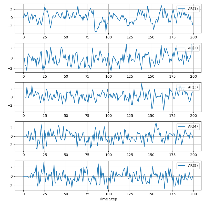
# Parameters for different AR processes
n_samples = 200
ar_processes = {
    "AR(1)": generate_ar_process(1, [0.7], 1, n_samples),
    "AR(2)": generate_ar_process(2, [0.6, -0.2], 1, n_samples),
    "AR(3)": generate_ar_process(3, [0.5, -0.3, 0.2], 1, n_samples),
    "AR(4)": generate_ar_process(4, [0.4, -0.4, 0.3, -0.1], 1, n_samples),
    "AR(5)": generate_ar_process(5, [0.3, -0.5, 0.4, -0.2, 0.1], 1, n_samples)
}

# Create a grid of subplots (5 rows, 1 column)
plt.figure(figsize=(8, 8))

for i, (label, process) in enumerate(ar_processes.items(), start=1):
    plt.subplot(5, 1, i) 
    plt.plot(process, label=label, linewidth=1.5)
    plt.grid(True)
    plt.legend(loc="upper right")

plt.xlabel("Time Step")
plt.tight_layout()
plt.show()

Stationarity in AR Models

For the AR process to be stationary, the following condition must hold:

• \(

  \phi_1

  < 1\) for AR(1);

• roots of the characteristic polynomial must lie outside the unit circle for AR(p).

If this condition is violated, the time series can become non-stationary (e.g., trending or diverging), which could lead to inaccurate forecasts.

Estimation of AR Models

To estimate the parameters \(\phi_1, \phi_2, \dots, \phi_p\) of the AR model, one commonly used method is Least Squares Estimation (LSE) (see my previous post), which minimizes the sum of squared differences between the observed values and the predicted values from the model.

Alternatively, for larger AR models, methods such as Maximum Likelihood Estimation (MLE) or Yule-Walker equations are used to estimate the coefficients. In addition, Bayesian learning can also be employed, see my paper Calibrating Car-Following Models via Bayesian Dynamic Regression .

Applications of AR Processes

Autoregressive processes are widely used in modeling time series data across various domains. Some common applications include:

1. Traffic Modeling: In traffic flow theory, AR models are used to predict traffic conditions such as car-following behaviors or congestion, based on past observations of speed or position.
2. Economics: AR models are used to model economic indicators such as inflation, stock prices, or GDP, where past values of these indicators can predict future values.
3. Finance: AR processes are used in financial markets to model stock returns, interest rates, and volatility, often in conjunction with other models like GARCH (Generalized Autoregressive Conditional Heteroskedasticity).
4. Engineering: In signal processing, AR models are used to model system dynamics, such as vibrations or electrical signals, where past behavior is used to predict future behavior.
5. Weather Forecasting: AR models can be applied to weather data to predict temperature or precipitation levels based on past measurements.

Advantages and Limitations of AR Processes

Advantages:

1. Simplicity: AR models are relatively easy to understand and implement.
2. Interpretability: The autoregressive coefficients provide direct insights into the influence of past values on the current state.
3. Efficiency: AR models are computationally efficient and well-suited for real-time forecasting.

Limitations:

1. Linear Assumption: AR models assume a linear relationship between past and current values, which may not always capture complex non-linear patterns.
2. Stationarity Requirement: AR models require the data to be stationary. Non-stationary data, such as trends or seasonality, must be transformed before using AR models.
3. Limited Memory: The AR model relies only on past values up to a fixed number of lags. This means that long-term dependencies may not be well captured unless higher-order AR models (AR(p)) are used.

My Research on AR Processes

(See Eqs. (8)-(10), then you will understand why we say “it involves rich information from several historical steps to make decisions for the current step instead of using only one historical step.”)

• Chengyuan Zhang, Wenshuo Wang, and Lijun Sun* (2024). Calibrating Car-Following Models via Bayesian Dynamic Regression. Transportation research part C: emerging technologies. (Accepted to ISTTT25 Special Issue) [TR PartC] [arXiv] [code] [presentation] [slides]