
Hidden Markov Model and Driving Behavior Modeling: From HMMs to Factorial HMMs to FHMM–IDM — a three–part primer
Published:
This post is part of a series that supports and promotes our recent document. It collects three parts into one page so readers can follow the full narrative from basic HMMs to a factorial model and then to an interpretable driving framework.
Unified notation used throughout
- Time index: \(t=1,\dots,T\)
- Observation: \(y_t\). In Part III we set \(y_t\) to the vehicle acceleration.
- Covariates (inputs): \(x_t\). In Part III we set \(x_t=[v_t,\,\Delta v_t,\,s_t]^\top\), where \(v_t\) is speed, \(\Delta v_t\) is closing speed (follower minus leader), and \(s_t\) is spacing.
- Latent state: \(z_t\in\{1,\dots,K\}\)
- Transition matrix: \(\Pi\in\mathbb{R}^{K\times K}\) with rows that sum to 1 and entries \(\Pi_{j,k}=p(z_t=k\mid z_{t-1}=j)\)
- Local evidence at time \(t\): \(\psi_t(k)=p(y_t\mid x_t,\theta_k)\)
- Shorthands: \(y_{1:T}=\{y_t\}_{t=1}^T\), \(x_{1:T}=\{x_t\}_{t=1}^T\), \(z_{1:T}=\{z_t\}_{t=1}^T\)
Part I. Hidden Markov Models, filtering vs smoothing vs prediction, and the forward–backward algorithm
HMM recap
An HMM couples a discrete Markov chain \(z_t\) to observations \(y_t\):
\[z_t\mid z_{t-1}\sim \mathrm{Cat}(\Pi_{z_{t-1},:}),\qquad y_t\mid x_t,\Theta,z_t \sim p(\,\cdot\mid x_t,\theta_{z_t}).\]The joint distribution is
\[p(y_{1:T},z_{1:T}\mid x_{1:T},\Theta,\Pi)= p(z_1)\,\psi_1(z_1)\prod_{t=2}^T \Pi_{z_{t-1},z_t}\,\psi_t(z_t).\]Tasks: filtering, smoothing, prediction
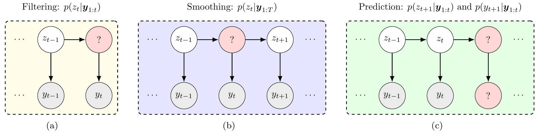
- Filtering computes \(p(z_t\mid y_{1:t},x_{1:t})\). This is causal and uses data up to time \(t\).
- Smoothing computes \(p(z_t\mid y_{1:T},x_{1:T})\). This is acausal and uses the full sequence.
- Prediction computes \(p(z_{t+1}\mid y_{1:t},x_{1:t})\) or \(p(y_{t+1}\mid y_{1:t},x_{1:t+1})\).
Forward–backward definitions
We use the standard unnormalized messages
\[\alpha_t(k)=p(y_{1:t}\!,x_{1:t}, z_t=k),\qquad \beta_t(k)=p(y_{t+1:T}\!,x_{t+1:T}\mid z_t=k).\]These satisfy \(p(y_{1:T}\!,x_{1:T}, z_t=k)=\alpha_t(k)\,\beta_t(k)\). The smoothed marginal is
\[\gamma_t(k)=p(z_t=k\mid y_{1:T},x_{1:T})= \frac{\alpha_t(k)\,\beta_t(k)}{\sum_{j=1}^K \alpha_t(j)\,\beta_t(j)}.\]Forward pass
Initialization and recursion:
\[\alpha_1(k)=p(z_1=k)\,\psi_1(k),\qquad \alpha_t(k)=\psi_t(k)\sum_{j=1}^K \alpha_{t-1}(j)\,\Pi_{j,k},\quad t\ge 2.\]Backward pass
\[\beta_T(k)=1,\qquad \beta_t(k)=\sum_{j=1}^K \Pi_{k,j}\,\psi_{t+1}(j)\,\beta_{t+1}(j),\quad t\le T-1.\]Practical notes
- Use scaling or log space to avoid numerical underflow. For example, normalize \(\alpha_t\) and \(\beta_t\) at each step and track the scaling constants to recover sequence likelihoods.
- The expected two–slice counts \(\xi_t(j,k)\propto \alpha_{t-1}(j)\,\Pi_{j,k}\,\psi_t(k)\,\beta_t(k)\) are useful for EM and for estimating transition matrices.
- For state sampling, draw \(z_t\sim \mathrm{Cat}(\gamma_t)\).
Part II. Factorial HMM: separating behavior and scenario
A factorial HMM (FHMM) uses multiple latent chains that act in parallel. In our setting we use two:
- A behavior factor \(z_t^{[B]}\in\{1,\dots,K^{[B]}\}\).
- A scenario factor \(z_t^{[S]}\in\{1,\dots,K^{[S]}\}\).
The joint state is \(z_t=(z_t^{[B]},z_t^{[S]})\) in the product space \(\mathcal{Z}=\{1,\dots,K^{[B]}\}\times\{1,\dots,K^{[S]}\}\).
| Let \(k=(k^{[B]},k^{[S]})\) index a joint state. The transition matrix is $$\Pi\in\mathbb{R}^{ | \mathcal{Z} | \times | \mathcal{Z} | }$$ with rows that sum to 1: |
Factorized emissions and joint evidence
We model two pieces of local evidence that multiply:
- Behavior evidence \(\psi_t^{[B]}(k^{[B]})=p(y_t\mid x_t,\Theta, z_t^{[B]}=k^{[B]})\).
- Scenario evidence \(\psi_t^{[S]}(k^{[S]})=p(x_t\mid z_t^{[S]}=k^{[S]},\mu_x,\Lambda_x)\).
The joint local evidence for \(k=(k^{[B]},k^{[S]})\) is
\[\Psi_t(k)=\psi_t^{[B]}(k^{[B]})\;\psi_t^{[S]}(k^{[S]}).\]The sequence likelihood factorizes as
\(p(y_{1:T},x_{1:T}\mid z_{1:T},\cdot)=\prod_{t=1}^T \Psi_t(z_t)\).
Inference
Treat the joint index \(k\) as a single categorical state of size \(|\mathcal{Z}|=K^{[B]}K^{[S]}\) and run the same forward–backward recursions with \(\psi_t\) replaced by \(\Psi_t\):
\[\alpha_t(k)=\Psi_t(k)\sum_{k'}\alpha_{t-1}(k')\,\Pi_{k',k},\qquad \beta_t(k)=\sum_{k'}\Pi_{k,k'}\,\Psi_{t+1}(k')\,\beta_{t+1}(k').\]Smoothing and sampling then follow from Part I. When the transition matrix factorizes (for example with Kronecker structure), efficient message passing is possible, but the basic presentation above already works and keeps notation simple and unified.
Part III. FHMM–IDM: a factorial HMM with interpretable driving physics
 In this part we instantiate the FHMM with an interpretable physics–based emission for driver acceleration and a Gaussian model for traffic scenarios. We keep the same notation.
- Set \(y_t=a_t\) to be the follower’s acceleration.
- Set \(x_t=[v_t,\,\Delta v_t,\,s_t]^\top\), where \(v_t\) is the follower’s speed, \(\Delta v_t\) is closing speed (follower minus leader), and \(s_t\) is spacing.
Behavior factor: IDM emission for acceleration
We use the Intelligent Driver Model (IDM) as the mean function for acceleration:
\[\mathrm{IDM}(x_t;\theta)=a_{\max}\left[1-\left(\frac{v_t}{v_f}\right)^{\delta}-\left(\frac{s^*}{s_t}\right)^2\right], \qquad s^*=s_0+v_t T+\frac{v_t\,\Delta v_t}{2\sqrt{a_{\max} b}}.\]The parameter set is \(\theta=\{v_f, s_0, T, a_{\max}, b, \delta\}\). In many applications \(\delta\) is fixed (for example \(\delta=4\)).
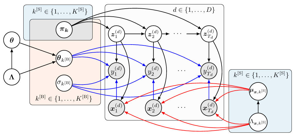
Let the behavior chain pick one of \(K^{[B]}\) parameter sets \(\{\theta_{k^{[B]}}\}\) and a corresponding noise scale:
\[a_t\mid x_t, z_t^{[B]}=k^{[B]}\sim \mathcal{N}\Big(\mathrm{IDM}(x_t;\theta_{k^{[B]}}),\; \sigma^2_{k^{[B]}}\Big).\]Scenario factor: a distribution for inputs
We model the distribution of inputs with a Gaussian for each scenario state:
\[x_t\mid z_t^{[S]}=k^{[S]}\sim \mathcal{N}\big(\mu_{x,k^{[S]}},\; \Lambda_{x,k^{[S]}}^{-1}\big).\]This captures typical speed, closing speed, and spacing patterns that co–occur in a scenario, for example free–flow, steady following, acceleration, deceleration, and near–stop.
Joint evidence and message passing
The joint local evidence is
\[\Psi_t\big(k^{[B]},k^{[S]}\big)= \underbrace{\mathcal{N}\big(a_t\,\big|\,\mathrm{IDM}(x_t;\theta_{k^{[B]}}),\sigma^2_{k^{[B]}}\big)}_{\psi_t^{[B]}(k^{[B]})}\; \underbrace{\mathcal{N}\big(x_t\,\big|\,\mu_{x,k^{[S]}},\Lambda_{x,k^{[S]}}^{-1}\big)}_{\psi_t^{[S]}(k^{[S]})}.\]Forward–backward then proceeds exactly as in Part II on the joint index \(k=(k^{[B]},k^{[S]})\), which yields smoothed posteriors \(\gamma_t(k)\) and expected two–slice statistics \(\xi_t(k',k)\).
Bayesian learning choices (a compact view)
A convenient set of priors that keeps conjugacy where possible:
- Rows of \(\Pi\): independent Dirichlet priors.
- Scenario parameters \((\mu_{x,k^{[S]}},\Lambda_{x,k^{[S]}})\): Normal–Wishart.
- Behavior noise scales \(\sigma^2_{k^{[B]}}\): Inverse–Gamma.
- IDM parameters \(\theta_{k^{[B]}}\): log–normal or weakly informative normals on a suitable transform.
The joint prior factorizes as
\[p(\Omega)=p(\Pi)\,p(\{\sigma^2\})\,p(\{\theta\})\,p(\{\mu_x,\Lambda_x\}).\]Posterior inference can be done with EM or with MCMC. Either way, forward–backward appears inside the inner loop for computing the required expectations.
What this buys us
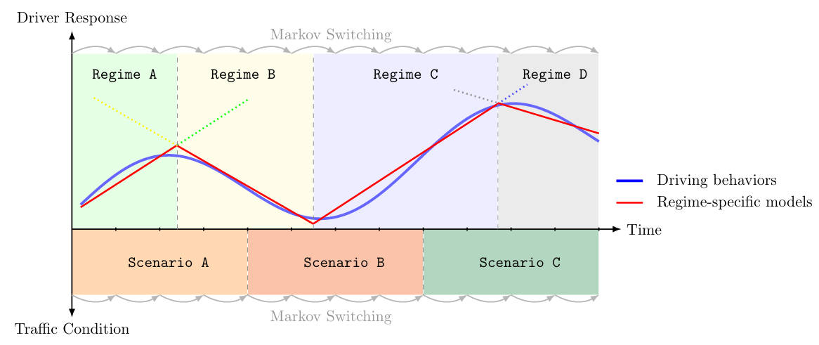
- The behavior chain provides interpretable regimes through \(\theta_{k^{[B]}}\), which are parameterizations of a physics model rather than opaque labels.
- The scenario chain explains context dynamics in \(x_t\), which reduces confounding and helps identify when similar accelerations arise from different contexts.
- Together these pieces allow filtering, smoothing, and prediction in a model that is both probabilistic and physically grounded, which benefits microscopic traffic simulation and downstream evaluation.
Quick reference: minimal pseudocode
Inputs: observations {y_t}, inputs {x_t}, transition Π, behavior params {θ_kB, σ2_kB}, scenario params {μx_kS, Λx_kS}

for t in 1..T:
    for kB in 1..K[B]:
        psiB[t,kB] = Normal(y_t | IDM(x_t; θ_kB), σ2_kB)
    for kS in 1..K[S]:
        psiS[t,kS] = Normal(x_t | μx_kS, Λx_kS^{-1})
    for (kB,kS) in product:
        Psi[t,kB,kS] = psiB[t,kB] * psiS[t,kS]

# Forward
alpha[1,:] = prior .* Psi[1,:]; normalize
for t in 2..T:
    alpha[t,:] = (alpha[t-1,:] @ Π) .* Psi[t,:]; normalize

# Backward
beta[T,:] = 1
for t in T-1..1:
    beta[t,:] = (Π * (Psi[t+1,:] .* beta[t+1,:])); normalize

# Smoothing
gamma[t,:] = normalize(alpha[t,:] .* beta[t,:])
Read More
For more detailed information on the mathematical formulation and applications of the GVF, refer to the original research paper:
- Chengyuan Zhang, Cathy Wu, and Lijun Sun*. Markov Regime-Switching Intelligent Driver Model for Interpretable Car-Following Behavior. arXiv preprint arXiv:2506.14762 (2025). [arXiv]