Time-series forecasting is a critical application of Gaussian Processes (GPs), as they offer a flexible and probabilistic framework for predicting future values in sequential data. GPs not only provide point predictions but also quantify uncertainty, making them particularly useful in scenarios where confidence in predictions is important.

1. Modeling Framework

To forecast time-series data, we use GPs to model the underlying function \( f(t) \) that generates the observations \( y_t \). The relationship is expressed as:

Here:

• \( f(t) \) is the latent function, which we assume follows a Gaussian Process:

  \[f(t) \sim \mathcal{GP}(m(t), k(t, t'))\]

• \( \epsilon \) is Gaussian noise with variance \( \sigma_\epsilon^2 \).

The goal is to infer the posterior distribution of \( f(t) \) given the observed data, and use this distribution to make predictions for future time points.

2. Steps in Forecasting

Step 1: Choose a Mean and Covariance Function

• The mean function \( m(t) \) typically defaults to zero unless prior knowledge suggests otherwise.
• The covariance function (kernel) \( k(t, t’) \) encodes assumptions about the data. Common kernels for time-series forecasting include:

  • Squared Exponential (SE) Kernel:

    \[k(t, t') = \sigma^2 \exp\left(-\frac{|t - t'|^2}{2 \ell^2}\right)\]

    This kernel produces smooth functions.

  • Matern Kernel:

    \[k(t, t') = \sigma^2 \frac{2^{1-\nu}}{\Gamma(\nu)} \left( \frac{\sqrt{2 \nu |t - t'|}}{\rho} \right)^\nu K_\nu \left( \frac{\sqrt{2 \nu |t - t'|}}{\rho} \right)\]

    It allows for varying levels of smoothness controlled by the parameter \( \nu \).

  • Periodic Kernel:

    \[k(t, t') = \sigma^2 \exp\left(-\frac{2 \sin^2(\pi |t - t'| / p)}{\ell^2}\right)\]

    Suitable for capturing periodic patterns.

  • Sum/Product Kernels: To combine different features (e.g., trend + seasonality).

Step 2: Fit the Gaussian Process

Given a dataset \( {t_1, t_2, \ldots, t_n} \) and observations \( {y_1, y_2, \ldots, y_n} \), the GP hyperparameters (e.g., kernel parameters such as length-scale and variance) are learned by maximizing the log marginal likelihood:

where \( \mathbf{K} \) is the covariance matrix computed using the kernel function.

Step 3: Make Predictions

For new time points \( \mathbf{t}_{*} \), the GP provides the posterior predictive distribution:

where:

Here:

• \( \mathbf{K}_{*} \) is the covariance between training and test points.
• \( \mathbf{K}_{**} \) is the covariance among test points.

3. Handling Specific Challenges in Time-Series

Trend and Seasonality

By combining kernels, GPs can capture complex behaviors in time-series data:

• Trend: Modeled with an RBF or Matern kernel.
• Seasonality: Modeled with a periodic kernel.

The combined kernel might look like:

Irregularly Spaced Data

GPs handle irregularly spaced time points naturally because the kernel operates on the pairwise distances between points.

Uncertainty in Long-Term Forecasting

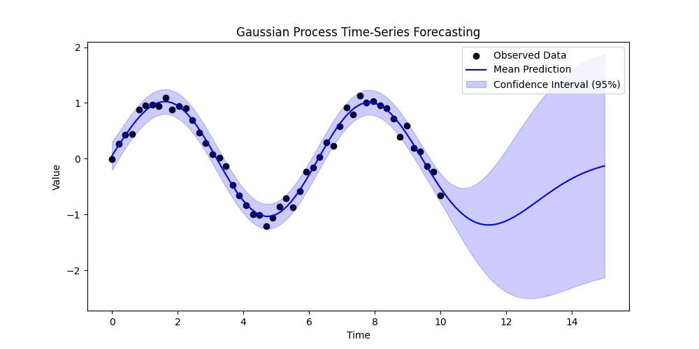
In long-term forecasts, GPs reflect increasing uncertainty by widening the confidence intervals as predictions are made further into the future.

4. Advantages of Using Gaussian Processes

• Uncertainty Quantification: GPs provide confidence intervals for predictions, which are valuable in decision-making.
• Flexibility: GPs can model non-linear relationships and adapt to various patterns in time-series data.
• Non-parametric Nature: GPs make minimal assumptions about the underlying function, allowing them to capture a wide range of behaviors.

5. Limitations and Solutions

Limitation: Computational Cost

• GPs scale cubically with the number of data points (\( \mathcal{O}(n^3) \)) due to matrix inversion.
• Solution: Use sparse approximations, such as inducing point methods, to reduce computational complexity.

Limitation: Kernel Selection

• Choosing the right kernel can be challenging and requires domain expertise.
• Solution: Use automatic relevance determination (ARD) or composite kernels to automate and refine kernel selection.

6. Example: Forecasting with Python

Here is a simple example of time-series forecasting using the scikit-learn library in Python:

import numpy as np
import matplotlib.pyplot as plt
from sklearn.gaussian_process import GaussianProcessRegressor
from sklearn.gaussian_process.kernels import RBF, WhiteKernel

# Generate synthetic time-series data
np.random.seed(37)
t = np.linspace(0, 10, 50)[:, None]  # Time points
y = np.sin(t).ravel() + 0.1 * np.random.randn(50)  # Observations

# Define the kernel (RBF + WhiteKernel for noise)
kernel = RBF(length_scale=1.0) + WhiteKernel(noise_level=0.1)

# Fit the Gaussian Process
gp = GaussianProcessRegressor(kernel=kernel, n_restarts_optimizer=10)
gp.fit(t, y)

# Predict for new time points
t_pred = np.linspace(0, 15, 100)[:, None]
y_pred, y_std = gp.predict(t_pred, return_std=True)

# Plot the results
plt.figure(figsize=(10, 5))
plt.scatter(t, y, c='k', label="Observed Data")
plt.plot(t_pred, y_pred, 'b-', label="Mean Prediction")
plt.fill_between(
    t_pred.ravel(),
    y_pred - 2 * y_std,
    y_pred + 2 * y_std,
    color='blue',
    alpha=0.2,
    label="Confidence Interval (95%)",
)
plt.legend()
plt.title("Gaussian Process Time-Series Forecasting")
plt.xlabel("Time")
plt.ylabel("Value")
plt.show()

7. Conclusion

Gaussian Processes provide a flexible, interpretable, and probabilistic framework for time-series forecasting. They excel in scenarios where uncertainty quantification is crucial and where the underlying patterns in the data may be non-linear or complex. Although computational challenges exist, advances in sparse approximations and scalable implementations have made GPs increasingly practical for real-world time-series applications.

By choosing appropriate kernels and leveraging their probabilistic nature, GPs offer powerful insights into temporal patterns and predictive uncertainty, making them a valuable tool in time-series analysis.