A Detailed Introduction to Gaussian Velocity Fields (GVF) Based on Gaussian Processes

In autonomous driving, modeling and understanding the interactions between the ego vehicle and its surrounding vehicles is crucial for safe and efficient navigation. One important challenge is dealing with varying traffic densities and dynamic environments, where the number of surrounding vehicles can fluctuate. Traditional models, which rely on a fixed number of surrounding vehicles, may struggle in such conditions.

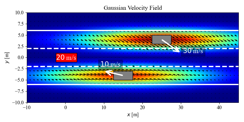
A promising approach to address this challenge is the concept of the Gaussian Velocity Field (GVF). The GVF is a probabilistic model that captures the velocity distribution of surrounding vehicles, enabling the ego vehicle to understand the dynamic interactions without depending on the exact number of nearby vehicles. In this post, we provide a detailed introduction to the GVF, including its mathematical formulation and its advantages for autonomous driving applications.

The Key Aim of Gaussian Velocity Fields

The primary goal of constructing a Gaussian Velocity Field is to represent the surrounding driving environment in a way that maintains consistent dimensionality regardless of the number of surrounding vehicles. This feature is crucial in dynamic traffic conditions where the number of nearby vehicles can vary significantly. The GVF provides a smooth, continuous, and scalable representation of velocity that adapts to the changing environment, making it a powerful tool for autonomous vehicle decision-making.

Why is this Important?

• In real-world scenarios, the number of vehicles surrounding an autonomous vehicle is not fixed—it fluctuates based on traffic conditions. The ability to represent this dynamically changing number of vehicles without reconfiguring the model is essential for maintaining real-time performance.

• Traditional models may struggle to handle such variability because they often require a fixed number of vehicles or states. The GVF, on the other hand, uses Gaussian Processes (GPs) to model the interactions in a nonparametric way, meaning the dimensionality of the feature remains constant even as the number of surrounding vehicles changes.

Mathematical Framework of Gaussian Velocity Fields

1. Gaussian Processes (GPs)

At the core of the Gaussian Velocity Field is the use of Gaussian Processes (GPs), which provide a probabilistic approach to modeling spatial and temporal relationships. A Gaussian Process is a distribution over functions, where any finite collection of function values follows a multivariate normal distribution. In the context of GVFs, the function we model is the velocity field at various locations in space.

Mathematically, a GP is defined as:

where:

• \(v(\mathbf{x})\) is the velocity at location \(\mathbf{x}\) in space.
• \(m(\mathbf{x})\) is the mean function, often assumed to be zero unless prior knowledge suggests otherwise.
• \(k(\mathbf{x}, \mathbf{x}')\) is the covariance function (or kernel) that encodes the relationship between velocities at different spatial locations \(\mathbf{x}\) and \(\mathbf{x}'\).

2. Constructing the Gaussian Velocity Field

Given the positions \(\mathbf{x}_i\) and velocities \(v_i\) of the surrounding vehicles, the goal is to model the velocity field \(v(\mathbf{x})\) as a Gaussian Process.

Input Data:

• \(\mathbf{X} = \{ \mathbf{x}_1, \mathbf{x}_2, \dots, \mathbf{x}_N \}\) are the positions of the surrounding vehicles.
• \(\mathbf{v} = \{ v_1, v_2, \dots, v_N \}\) are the observed velocities of these vehicles at the respective positions.

Posterior Distribution:

Once we have observed data at certain locations \(\mathbf{x}_i\), we can make predictions about the velocity at new, unobserved locations \(\mathbf{x}_*\) using the posterior distribution of the Gaussian Process. This is given by:

where:

• \(\mu_*\) is the predicted mean velocity at \(\mathbf{x}_*\):

  \[\mu_* = \mathbf{k}_*^\top \mathbf{K}^{-1} \mathbf{v}\]

• \(\Sigma_*\) is the predictive variance (uncertainty) at \(\mathbf{x}_*\):

  \[\Sigma_* = k(\mathbf{x}_*, \mathbf{x}_*) - \mathbf{k}_*^\top \mathbf{K}^{-1} \mathbf{k}_*\]

Here:

• \(\mathbf{k}_*\) is the covariance vector between the new test location \(\mathbf{x}_*\) and all observed locations \(\mathbf{x}_i\).
• \(\mathbf{K}\) is the covariance matrix of the observed locations \(\mathbf{X}\).

This posterior distribution allows us to make predictions about the velocity at any point \(\mathbf{x}_*\), along with a measure of uncertainty, which is crucial for decision-making in dynamic environments. Please see my other post on Gaussian Processes (GP) for Time Series Forecasting for more details on GPs.

3. Maintaining Dimensional Consistency

One of the challenges in modeling dynamic environments is the changing number of surrounding vehicles. The GVF addresses this by not relying on the exact number of surrounding vehicles. Instead of creating a fixed-dimensional feature vector, the GVF is constructed as a field that represents velocity in a smooth, continuous manner.

• Fixed Dimensionality: The dimensionality of the Gaussian Velocity Field remains constant, even as the number of surrounding vehicles changes. This is achieved by representing the environment as a field that is modeled probabilistically, where the Gaussian Process can scale to accommodate any number of vehicles without needing to adjust the model.

• Scalable to Traffic Variability: Whether there are few or many vehicles, the dimensionality of the GVF feature vector remains consistent. This makes the model robust to varying traffic conditions, providing continuous predictions of velocity for the ego vehicle to act upon.

Advantages of Gaussian Velocity Fields

1. Probabilistic and Adaptive:
   • By using Gaussian Processes, GVFs capture both the predicted velocities and their associated uncertainties. This enables the ego vehicle to make safe decisions even in uncertain environments.
2. Consistent Representation:
   • The GVF allows for a consistent representation of the surrounding environment, independent of the number of surrounding vehicles. This is achieved through the Gaussian Process framework, which maintains the dimensionality of the feature space.
3. Smooth and Scalable:
   • The velocity field is smooth and scalable, adapting to the traffic environment and providing accurate predictions in both low-traffic and high-traffic situations.
4. Efficient Representation:
   • The GVF is efficient in that it allows the ego vehicle to process spatial interactions between surrounding vehicles as a continuous field rather than discrete features, thus improving performance in dynamic scenarios.

Conclusion

The Gaussian Velocity Field (GVF) is a powerful approach for modeling the dynamic interactions between the ego vehicle and its surrounding vehicles in autonomous driving scenarios. Its main advantage is its ability to represent the velocity field in a probabilistic and scalable way, maintaining consistent dimensionality despite the changing number of vehicles. This makes it particularly useful for modeling multivehicle interactions in environments where traffic density varies, providing a more robust and flexible framework for real-time decision-making in autonomous systems.

Read More

For more detailed information on the mathematical formulation and applications of the GVF, refer to the original research paper:

1. Chengyuan Zhang, Jiacheng Zhu, Wenshuo Wang*, and Junqiang Xi (2021). Spatiotemporal learning of multivehicle interaction patterns in lane-change scenarios. IEEE Transactions on Intelligent Transportation Systems. [IEEE TITS] [arXiv] [code] [demo] [project website]
2. Wenshuo Wang, Chengyuan Zhang, Pin Wang, and Ching-Yao Chan* (2020, October). Learning Representations for Multi-Vehicle Spatiotemporal Interactions with Semi-Stochastic Potential Fields. In 2020 IEEE Intelligent Vehicles Symposium (IV) (pp. 1935-1940). IEEE. [IEEE IV20’]
3. Chengyuan Zhang, Jiacheng Zhu, Wenshuo Wang, and Ding Zhao* (2019, October). A general framework of learning multi-vehicle interaction patterns from video. In 2019 IEEE Intelligent Transportation Systems Conference (ITSC) (pp. 4323-4328). IEEE. [IEEE ITSC19’][arXiv][project website]

• Code: [Github].
• Project website: [web].
• Watch the demos via: [YouTube] or [Bilibili].

If you find the codes or paper useful for your research, please cite our paper:

@article{zhang2021spatiotemporal,
      title={Spatiotemporal learning of multivehicle interaction patterns in lane-change scenarios},
      author={Zhang, Chengyuan and Zhu, Jiacheng and Wang, Wenshuo and Xi, Junqiang},
      journal={IEEE Transactions on Intelligent Transportation Systems},
      year={2021},
      publisher={IEEE}
}

@inproceedings{zhang2019general,
  title={A general framework of learning multi-vehicle interaction patterns from video},
  author={Zhang, Chengyuan and Zhu, Jiacheng and Wang, Wenshuo and Zhao, Ding},
  booktitle={2019 IEEE Intelligent Transportation Systems Conference (ITSC)},
  pages={4323--4328},
  year={2019},
  organization={IEEE}
}

@inproceedings{wang2020learning,
  title={Learning Representations for Multi-Vehicle Spatiotemporal Interactions with Semi-Stochastic Potential Fields},
  author={Wang, Wenshuo and Zhang, Chengyuan and Wang, Pin and Chan, Ching-Yao},
  booktitle={2020 IEEE Intelligent Vehicles Symposium (IV)},
  pages={1935--1940},
  year={2020},
  organization={IEEE}
}